
WhatsApp Chat Analysis (#1)
Ege Or, 12 July 2018
WhatsApp, the new-school messaging application. New trend! Facebook’s main squeeze. After many years under the SMS authority, it somehow saved our lives. Besides them all users are told that their data are protected by encription. Hereinafter, I would not expand the introduction. I’d like to ask just a short question: Do you wonder the structure of your conversations? In other words, do you want to learn who answers back late, the most frequent words, or which days you have more conversation? If your answer is yes, then you can follow the next parts of my post.
Exporting the Chat
Firstly, you need to send your chat backup to your email. To send your backup file, in your app you can find export chat option. These steps are for iOS. If you use Android, it is also similar. Just when you export your chat, don’t export your media files.
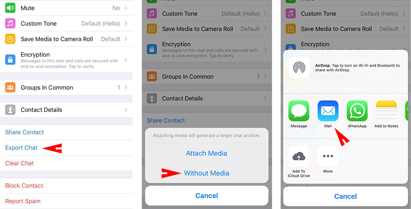
* For sure, I don’t disclose my private conversations. I just show the codes.
Import into R
Let us start doing something. For instance, we can import your convo into R. We cannot import the txt file regularly. We have to do some modification onto the regular read.table method. We have two people in our conversation: Person 1, Person 2.
require(data.table)
require(dplyr)

Sys.setlocale("LC_ALL", 'en_US.UTF-8')

setwd("...") # File path

convo <- fread("your_file.txt",fill = TRUE, header = FALSE,sep = "]") # Please modify your filename as yours

# If fread doesn't work, you can try the following way
# require(stringr)
# convo <- data.frame(tstrsplit(readLines("your_file.txt"),
#                           "]", type.convert=TRUE, names=TRUE, keep=1:2),
#               stringsAsFactors=FALSE)

convo$V1 <- gsub("\\[|\\,", "", convo$V1) # Separate into columns
names(convo) <- c("date","text")

# My timezone is GMT+1, you can modify according to your timezone.
convo$date <- as.POSIXct(convo$date, format = "%d/%m/%Y %H:%M:%S", tz = "Europe/Berlin")

convo$who <- ifelse(grepl("Person 1: ", x = a$text), "P1", "P2")

# Convert your omitted media files into understandable format
convo$text <- gsub("audio omitted", "audio_file", convo$text)
convo$text <- gsub("GIF omitted","gif_file",convo$text)
convo$text <- gsub("image omitted","image_file",convo$text)
convo$text <- gsub("video omitted","video_file",convo$text)
convo$text <- gsub("document omitted","pdf_file",convo$text)
Now, data is almost ready and you are able to see who sent more messages:
summ <- convo %>%
  group_by(who) %>%
  summarise(messages = table(who))
You can see the answering delay by following chunk:
require(xts)
convo_xts <- convo

# Person 2 is called 0, Person 1 is 1
convo_xts$who <- ifelse(convo_xts$who == "Person 2", 0, 1)
convo_xts <- convo_xts[,c("date","who")]
convo_xts <- xts(convo_xts[,-1],convo_xts[,1])

colnames(convo_xts) <- "who"
convo_xts$ans <- diff.xts(convo_xts$who)

p1_ans <- convo_xts[which(convo_xts$ans == 1),]
p2_ans <- convo_xts[which(convo_xts$ans == -1),]

p2_ans$diff <- diff.xts(index(p2_ans))
p1_ans$diff <- diff.xts(index(p1_ans))

x <- merge.xts(p2_ans[,3],p1_ans[,3])
colnames(x) <- c("p2_ans","p1_ans")

# Message latency plot for Person 2
plot.xts(na.omit(x$p2_ans), main = "Answering latency (Person 2)", col = c("pink"),
         grid.ticks.on = "months", grid.ticks.lty = 2, grid.ticks.lwd = 0.5)
I can get the following plot after I analyze the answering latency of my friend. You can easily see the time when we did not talk and we talk frequently between us, right here: 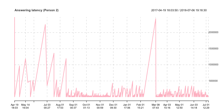
If you try to find a way to see the average answering time and average word number for each messages, the following chunk may help you:
# Average answering time (in hours)
mean(p1_ans$diff[-1,])/(60*60)
mean(p2_ans$diff[-1,])/(60*60)
# Mean and maximum word number in one message for both people
p1 <- convo$text[which(convo$who == "Person 1")]
mean(sapply(strsplit(p1, " "), length))
max(sapply(strsplit(p1, " "), length))
p2 <- convo$text[which(convo$who != "Person 1")]
mean(sapply(strsplit(p2, " "), length))
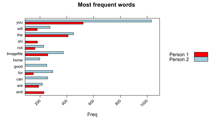
max(sapply(strsplit(p2, " "), length))Which words are used the most? We can write a simple function for it and see the result soon.
most_freq <- function(conversation){
  require(tm)
  docs0 <- Corpus(VectorSource(conversation)) # Turn the text into a corpus
  docs0 <- tm_map(docs0, content_transformer(tolower)) # All characters are lowercase
  docs0 <- tm_map(docs0, stripWhitespace) # Remove white spaces
  docs0 <- tm_map(docs0, removePunctuation) # Remove punctuation characters
  dtm0 <- TermDocumentMatrix(docs0)
  m0 <- as.matrix(dtm0)
  v0 <- sort(rowSums(m0),decreasing=TRUE)
  d0 <- data.frame(word = names(v0),freq=v0)
  d0 <- head(d0,10) # The most frequent 10 words
  d0 <- arrange(d0,-freq)
  return(d0)
}

p1_most_freq <- most_freq(p1)
p2_most_freq <- most_freq(p2)

p1_most_freq$who <- as.factor("Person 1")
p2_most_freq$who <- as.factor("Person 2")

most_freq_all <- rbind(p1_most_freq,p2_most_freq)
most_freq_all <- most_freq_all[order(most_freq_all$freq,decreasing = T),]

# Plot for the most frequence words
require(lattice)
barchart(word ~ freq, data = most_freq_all, groups = who, col = c("red","light blue"),
         auto.key=list(space='right'),scales=list(x=list(rot=45)),
         par.settings=list(superpose.polygon=list(col=c("red","light blue"))),
         main = "Most frequent words", xlab = "Freq")
The most frequent words of each person is here. Person 1 and 2 use “you” word the most, but Person 2 is quite superior to type it than Person 1. Person 2 sends more image files than Person 1:
If you want to see the conversation in weekdays, you can try the following code:
convo$wday <- as.POSIXlt(convo$date)$wday # Working with weekdays needs POSIXlt format rather than POSIXct

summ_wday <- convo[,-c(1,2)] %>%
  group_by(wday,who) %>%
  summarise(table(wday))
colnames(summ_wday)[3] <- "freq"

summ_wday[which(summ_wday$wday == 0),1] <- 7 # I convert Sunday from 0 to 7

summ_wday$wday <- factor(summ_wday$wday,
                         levels = rev(sort(unique(summ_wday$wday))),
                         ordered = TRUE)

summ_wday <- as.data.frame(summ_wday)

barchart(as.factor(wday) ~ freq, data = summ_wday, groups = who, col = c("red","blue"),
         auto.key=list(space='right'),scales=list(x=list(rot=45)),
         par.settings=list(superpose.polygon=list(col=c("red","blue"))),
         main = "Conversation in weekays", xlab = "Freq")
and you can see a similar barplot as follows:
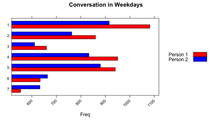
We can conclude them as these two people talked on Mondays the most and on Sundays the least. If you want to analyze deeply, I would recommend you to go further with sentiment analysis and/or (key)word extraction techniques. In my next posts, I am planning to show you how to classify the messages, how to understand/predict the owner of the messages. I would show some SVM techniques on R to define them.
Shiny Server on AWS
Ege Or, 30 June 2018
If you are familiar with R programming language, probably you are also acquainted with RStudio IDE and the packages. In order to create the interactive web applications based on R programming language, RStudio provides us again an amazing tool: Shiny. There are a bunch of examples for Shiny here.
However, today’s topic is not introduction to Shiny. I would like to tell you how to install RStudio and Shiny on your Amazon AWS EC2 instances, simply, and would try to explain apprehensibly. In my opinion, this process does not cause a lot of work. If you are on any of those Unix-like OS, this would not be that hard even. However, if you use Windows, you should struggle for some additional steps, such as PuTTY interface.
Here, I think I have to mention about some features of AWS EC2 virtual machines. There are various types of machines they provide, and the more powerful instances are directly proportionate to its fee. From the basic usage purpose to huge computational power, they have widespread types of instances. If you want to see a clear comparison of their virtual machines, you can visit their own website or you also can take a glance at this page.
* My next post “Let’s Shiny” will be related to this topic. I am planning writing a Shiny script on RStudio Server. If you want to follow my next post, I strongly recommend you to use RStudio and Shiny servers on AWS EC2 instances.
Launch an Ubuntu Instance
Firstly, we need to open an account on aws.amazon.com by providing your email address, username and your credit card information. Do not worry about it, because if you use any of the free tier services, Amazon does not withdraw any amount from your card (except the small provision fee). If you finish this step, please follow my next steps to have a free tier EC2 instance. If you don’t want to exceed the free tier limits in this post, you should choose t2.micro instance with any of the Linux OS. They give freely 750 hours of usage per month. 30 GiB of SSD capacity is also free. We will create our instances with respect to them for now.
Note: The following work is held on Mac OS X 10.12.6
On the top navigation bar, please click on the Services and find EC2 under the Compute section. 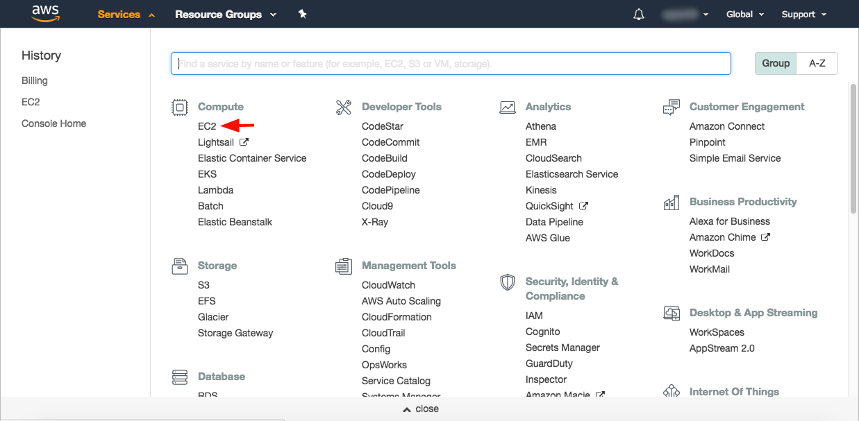
Step 1: Please choose your AMI (Amazon Machine Image) as Ubuntu Server 16.04 under the following options. 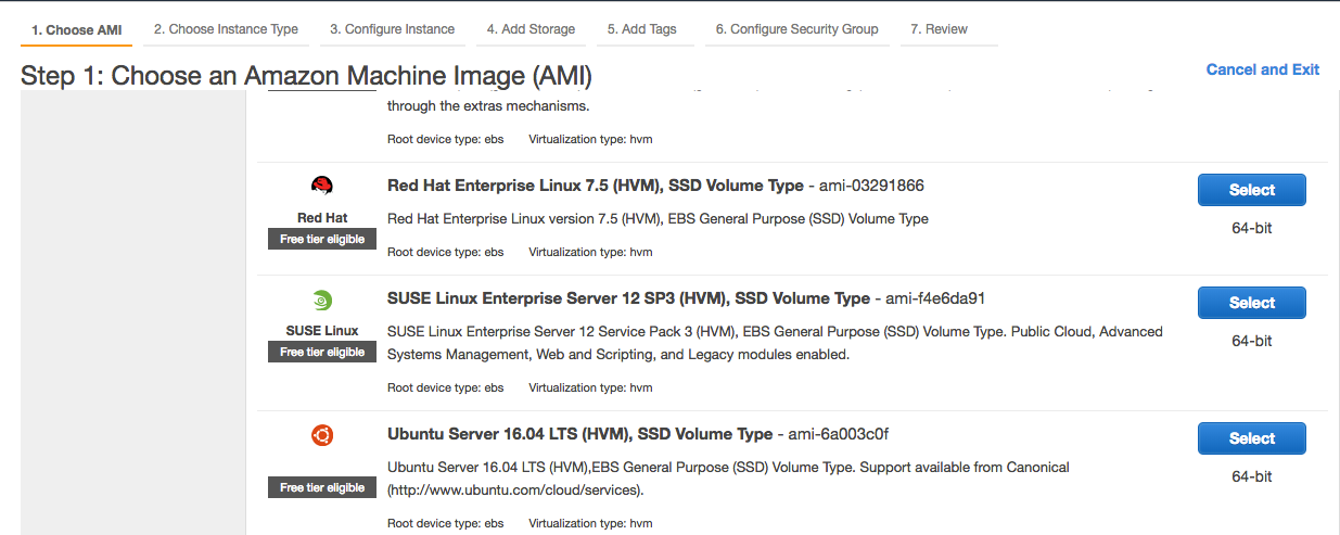
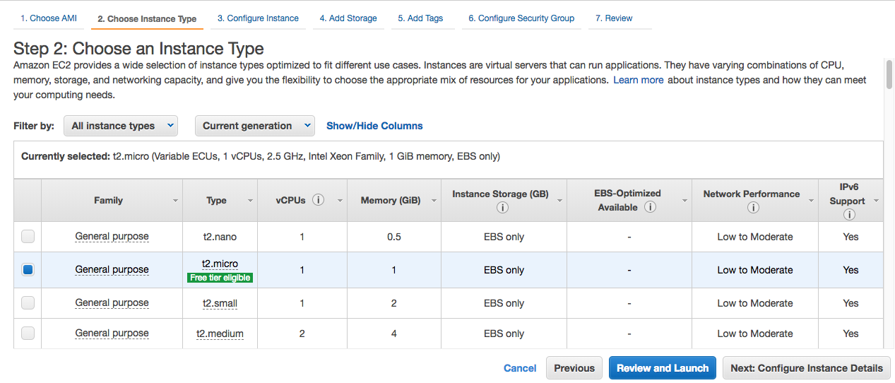
Step 2: Choose your instance type as t2.micro. Only this instance is eligible for free tier. However, if you need more powerful CPU, RAM, greater disk capacity or connection speed, you can choose a better service. Actually, I am using c5.large instance.
Step 3: We don’t need to configure any settings here. You can go to the next step. 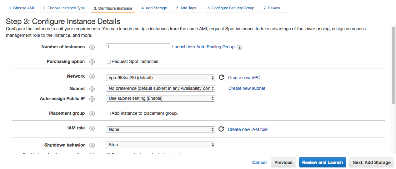
Step 4: Here, you may add 30 GiB of SSD storage as free tier. The minimum required capacity is 8 GiB. 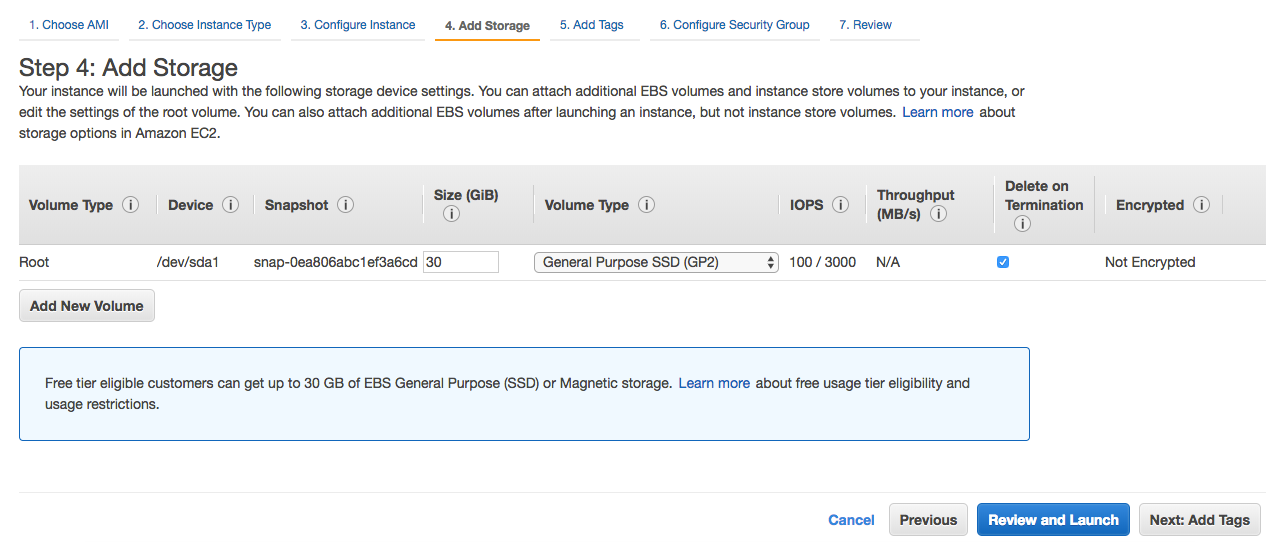
Step 5: I don’t add any tags here 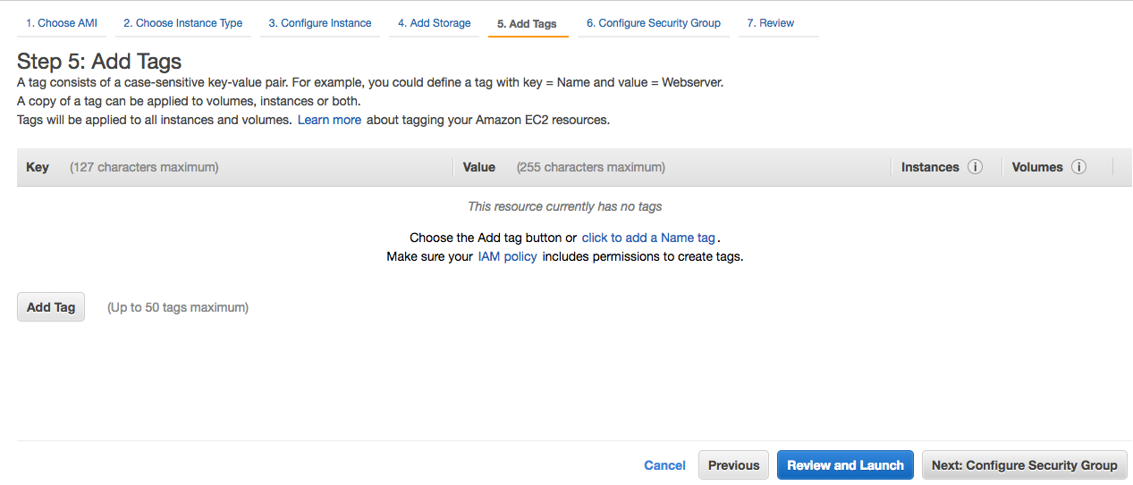
Step 6: Here is one of the most important steps. We have to add the security groups which will activate our RStudio Server and Shiny Server. RStudio and Shiny work on ports 8787 and 3838, respectively. You can exactly use the following settings to configure your security groups. These settings can also be changed later. 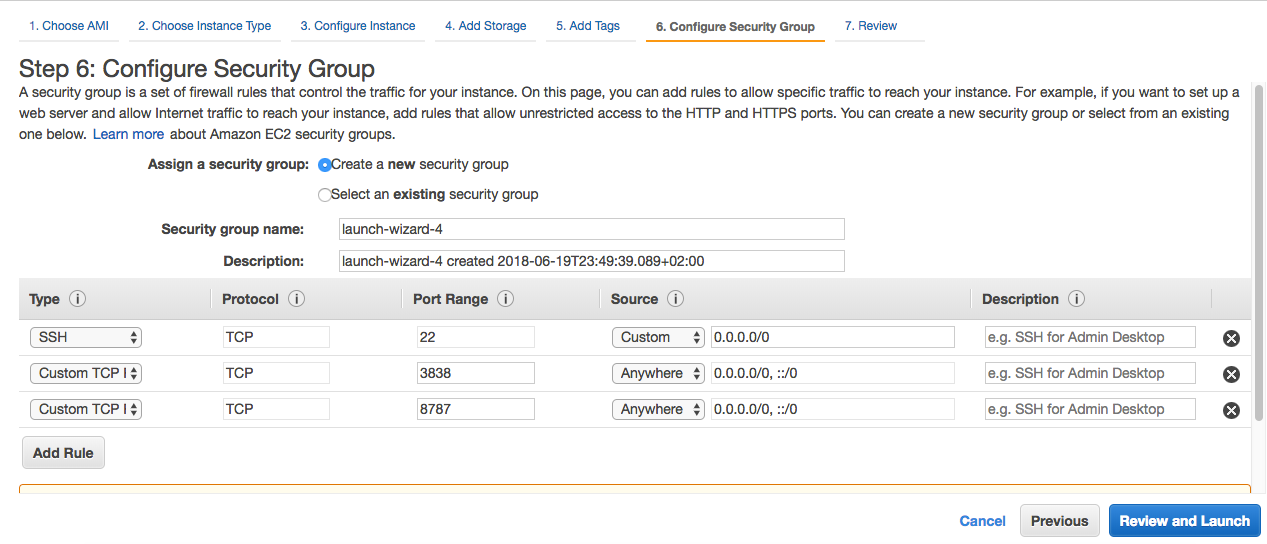
Step 7: In this step, you can review your instance and launch it. Finally! 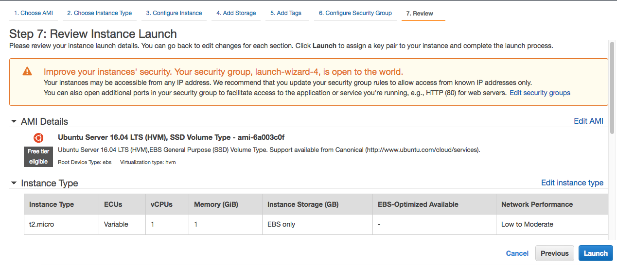
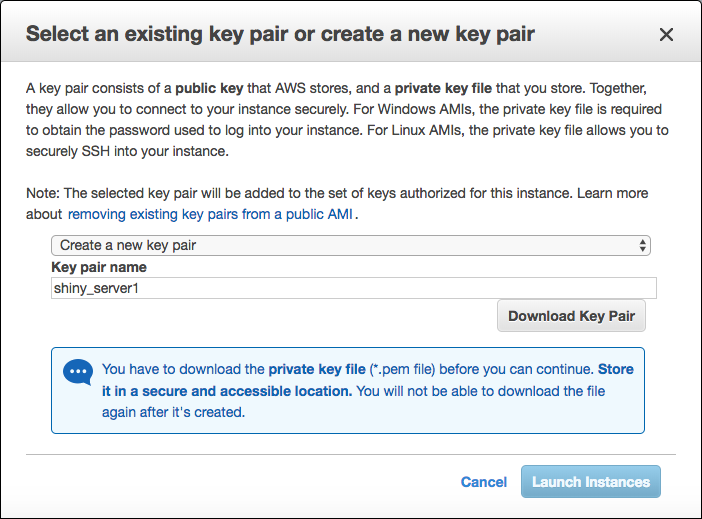
Step 8: Not yet! You need to create a key in order to have your access for this instance from your machine. Create a new pair key. (I assume you haven’t created any key previously.) Then download it to your machine. Please keep in your mind its file path and never lose mistakenly. You will need it. Otherwise, you would never connect to your instance from your local machine. I gave shiny_server1 name for my key. You can feel free about it.
Now your instance is being initialized. On the Sidebar the Instances link brings you the menu where you can see the list of all your instances, as follows: 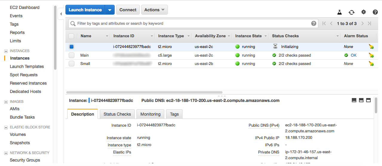
Congratulations! You have already created your EC2 instance. Hereinafter, we will only need to connect this instance. In order to realize that, we have to type some codes in Terminal. You can reach the Terminal by typing its name on Spotlight Search which you can open by ⌘+Space combination. Another way to open the Terminal is using its own file path: under /Applications/Utilities folder.
The code for your ssh connection is provided on AWS console. You can see the Connect button above, right next to the blue Launch Instance button. Click on it, and copy the following path to your clipboard.

Working With Terminal
I assume you are in front of the terminal now. You can type the following codes line-by-line (not all of them!). I guess that your key file is in your /Downloads folder.
Note: Do not copy $ signs.
$ cd Downloads
$ chmod 400 shiny_server1.pem
By chmod 400 code, the key file became an only owner can read, nobody can write and nobody can execute type. Then, you can paste the copied connection code from AWS console. My example is below:
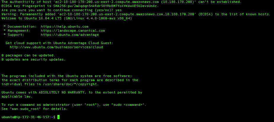
$ ssh -i "shiny_server1.pem" ubuntu@ec2-18-188-170-200.us-east-2.compute.amazonaws.comIf you are asked for anyhing, type yes. After you write the codes above, your screen should be as follows (may not be the same hacker theme):
So, welcome to your Amazon virtual machine. It’s time to install RStudio and Shiny on your server machine. Let us start. Please type the following codes line-by-line in your terminal:
$ sudo su -c "echo 'deb http://archive.linux.duke.edu/cran/bin/linux/ubuntu trusty/' >> /etc/apt/sources.list"
$ sudo apt-key adv --keyserver keyserver.ubuntu.com --recv-keys E084DAB9
$ sudo apt-get update
$ sudo apt-get upgrade
$ sudo apt-get dist-upgrade -y
Installation of R base:
$ sudo apt-get install r-base -yFrom now on, we install packages in following way, not in RStudio Server. Otherwise, packages can be installed only for one single user. Let’s install shiny and xts packages.
$ sudo su - \
  -c "R -e \"install.packages('shiny', repos='https://cran.rstudio.com/')\""
$ sudo su - \
  -c "R -e \"install.packages('xts', repos='https://cran.rstudio.com/')\""
Now, we visit RStudio Server’s page and find the link under Debian 8/Ubuntu section, 64-bit version. I give a sample code below, but it should not be forgotten that this is an updated site, codes/links will be changed.
$ sudo apt-get install gdebi-core
$ wget https://download2.rstudio.org/rstudio-server-1.1.453-amd64.deb
$ sudo gdebi rstudio-server-1.1.453-amd64.deb
Installation of RStudio Server needs the same process as previous one. It can be downloaded from Shiny Server’s website easily by following way:
Note: It should not be forgotten that this is an updated site, codes/links will be changed.
$ sudo apt-get install gdebi-core
$ wget https://download3.rstudio.org/ubuntu-14.04/x86_64/shiny-server-1.5.7.907-amd64.deb
$ sudo gdebi shiny-server-1.5.7.907-amd64.deb
Let’s visit the website where you created your Shiny Server. Firstly, to reach them you should check your Public IP address which is shown on your AWS console: 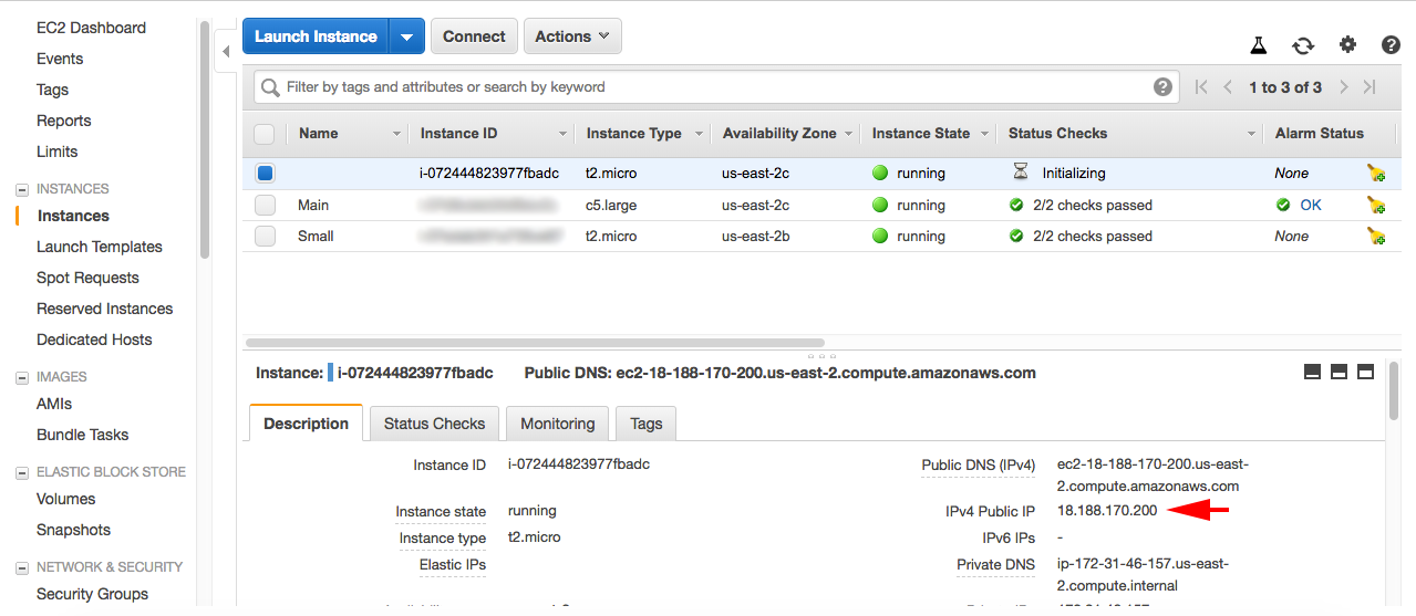
For instance, my public IP address is 18.188.170.200. If I enter the port 3838, I would reach to my Shiny Server and if I enter 8787, I would reach to my RStudio Server. I can write into the address line of my browser 18.188.170.200:3838 without any additional things, and I see the following page: 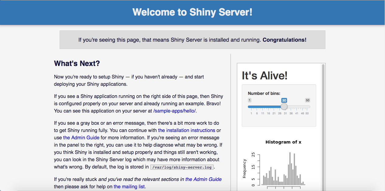
If you see the page above and also if you see the following box there, it means everything is fine, wszystko w porządku.
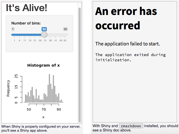
Also, don’t worry about the error above. You just need to install rmarkdown package lastly.
$ sudo su - \
  -c "R -e \"install.packages('rmarkdown', repos='https://cran.rstudio.com/')\""
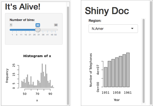
After you install rmarkdown package, boxes on the right side of Shiny Server page turn into the following style:
Congratulations once more! You activated your Shiny Server without any problems :)
Running RStudio Server on EC2
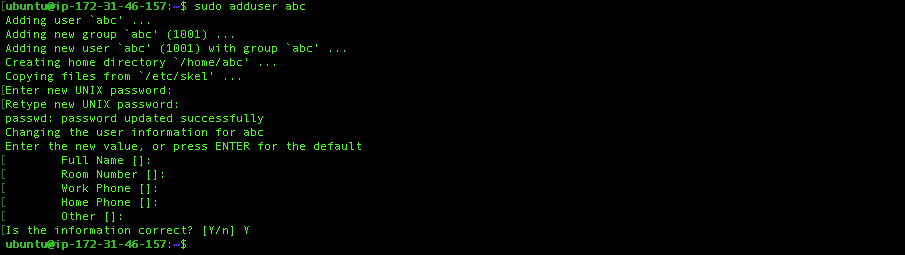
When you visit your RStudio Server page (http://your_public_ip:8787), it will ask you for the username and password. Before we go to your RStudio Server, we should create a new user on Ubuntu. Please follow the following code. I am adding the new user abc:
$ sudo adduser abcEnter your password. It doesn’t ask for any complex password. It will also ask you your name, phone number and so on. You can leave them empty. Then when it asks Is the information correct? Then type ‘Y’ and press enter.
If you created your new user, you are ready to give the privileges to this user. In order to do it, please type the following code, enter the editor and follow my instructions:
$ sudo vim /etc/sudoersPress I button,go down with your ↓ key and find the %sudo ALL=(ALL:ALL) ALL line and add the following line right below it.
%abc ALL=(ALL:ALL) ALL
Then, just press Esc button and type :wq! That’s all! It’s time to check your RStudio Server. In my example, my public IP address was 18.188.170.200 and I add my RStudio Server port into the end of this URL. When I enter 18.188.170.200:8787 address now, I can see a login panel. It shows that everything is fine. Write your username and password below:
Mission accomplished! Your Shiny Server and RStudio Server are ready. 
You can use all RStudio Server features in the same way as RStudio. Additionally, you will have an Upload option there. It would help you to upload the files from your local machine into your server. You don’t need to write any extra code to upload a file. I repeat it again and again but; if you need to install packages, do not install with install.packages() code in R. Use the following way:
$ sudo su - \
  -c "R -e \"install.packages('...', repos='...')\""
Possible Problems & Solutions
While you install packages, you may face with non-zero exit error. I have found couple of solutions in the long run. Especially, forecast, dplyr, devtools packages may not be installed due to this error. In order to work this error out, we can follow the codes below, in terminal:
# Possible solution for 'forecast' package
$ sudo apt-get install libxml2-dev
$ sudo su - \
  -c "R -e \"install.packages('forecast', repos='https://cran.rstudio.com/')\""
# Possible solution for 'dplyr' package
$ sudo apt-get update
$ sudo apt-get install software-properties-common
$ sudo add-apt-repository -y "ppa:marutter/rrutter"
$ sudo add-apt-repository -y "ppa:marutter/c2d4u"
$ sudo apt-get update
$ sudo apt-get install r-cran-readr
$ $ sudo su - \
-c "R -e \"install.packages('dplyr', repos='https://cran.rstudio.com/')\""# Possible solution for 'devtools' package
$ sudo apt-get -y build-dep libcurl4-gnutls-dev
$ sudo apt-get -y install libcurl4-gnutls-dev
$ sudo su - \
-c "R -e \"install.packages('devtools', repos='https://cran.rstudio.com/')\""Some packages may take long or they may overload the CPU and/or RAM. You can check your RAM usage by following code, simply:
$ sudo free -mIf you also want to see more detailed information for your RAM and CPU information, I would recommend you to install htop. It is a very efficient applocation in my opinion.
$ sudo apt-get install htopYou can also see the info about your CPU by following code:
$ sudo cat /proc/cpuinfoI am planning to tell about uploading your local Shiny apps into your Shiny server in my next post. I kind of divided this topic into two parts and it was the first one. After you read this long topic, I would thank you for your patience. Hope to see you in the next post. Keep working!
Fetching Twitter Data Using R
Ege Or, 6 June 2018
Everybody agrees that R is able to make various interesting things real. Catching the data on Twitter is one of these features. Here, I would like to mention about this. This topic was also one part of my master thesis. We can reach the data for tweets; however, one access code can only import 15000 tweets for each 15 minutes. If users need to remove this restriction, they should pay for it and it has come to my notice that, Twitter asks for really high price. Otherwise, they abort the process for 15 minutes. Also you are only able to see last 10 days’ tweets. Let’s start our work.
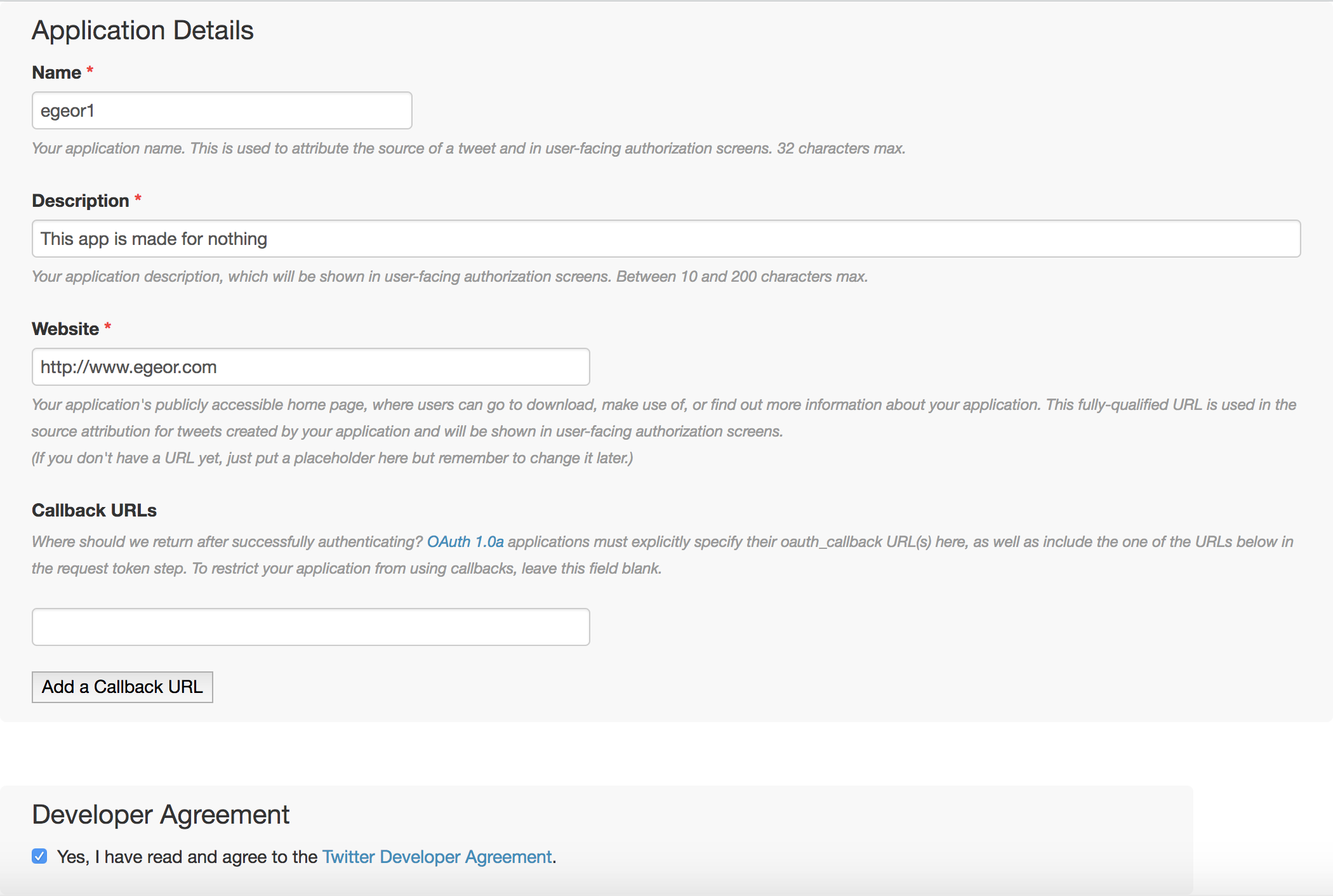
Firstly, you have to sign in application management website with your Twitter account. Here you can click on Create New App button. Then you would see the following screen and add the information in your own way and create the application.
If you see the following green box, that’s good news. Everything’s fine: 
Then please check out the Keys and Access Tokens tab there. You will find the info about your recently created application. 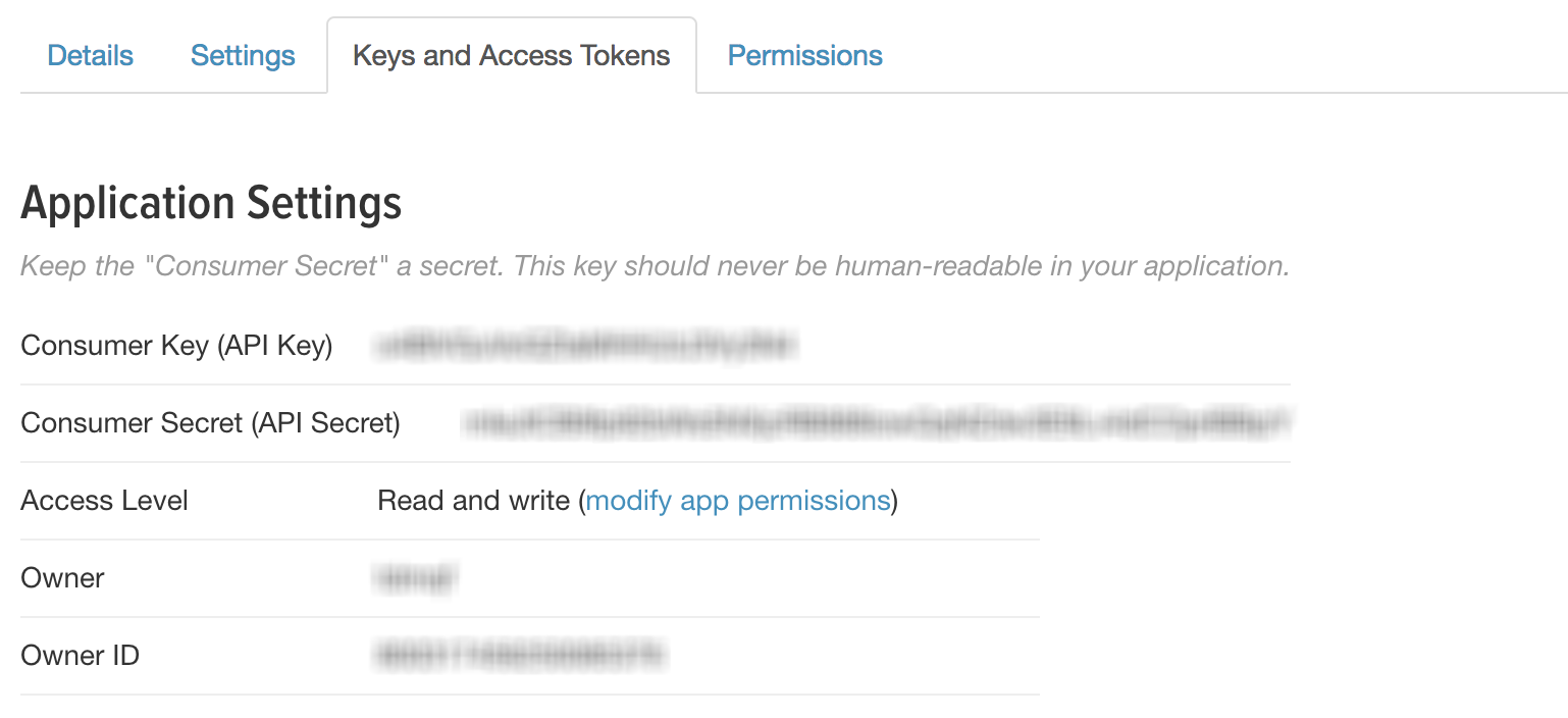
You have to keep your Consumer Key (API Key), Consumer Secret (API Secret) here. Then you can scroll down and click Create my access token button. Now, you can see all what you need there and keep your Access Token and Access Token Secret information somewhere.
Extraction of Tweets
From now on, you are going to need 4 keys and 1 package to authorize your API. And let’s go back to R and start scripting. We have to install twitteR package at first. There might be a problem for authorization and the solutions is easy. Just install base64enc package and call from the library. I add it into our chunk below, but this is just in case. You don’t have to:
install.packages("twitteR")
install.packages("base64enc")
require(twitteR)
require(base64enc)

# All keys are provided on your app information page
consumer_key <- '...'
consumer_secret <- "..."
access_token <- '...'
access_secret <- '...'
setup_twitter_oauth(consumer_key, consumer_secret, access_token, access_secret)
If you do this process the first time, it prints the following lines and here choose 1:
[1] "Using direct authentication"
Use a local file ('.httr-oauth'), to cache OAuth access credentials between R sessions?

1: Yes
2: No
That’s it! Now you can search a term in the posts, a specific user, you can reach whatever you want. Just one condition: if the account is not protected. Let’s start searching about the pharmaceutic company Pfizer Inc.. This company is also quoted on NYSE.
pfizer_ <- searchTwitter('pfizer',
                          lang = "en", # tweets only in English
                          since = substr(Sys.time()-60*60*24*3,1,16), # since 3 days ago
                          n = 1000) # maximum 1000 tweets
pfizer_ <- twListToDF(pfizer_)| text | favorited | favoriteCount | replyToSN | created | truncated | replyToSID | id | replyToUID | statusSource | screenName | retweetCount | isRetweet | retweeted | longitude | latitude |
|---|---|---|---|---|---|---|---|---|---|---|---|---|---|---|---|
| RT @AwesomeCapital: Nimbus Raises Another $65M from Lilly, Bill Gates, Pfizer,<U+00A0>others https://t.co/JhVYR7HQCU | FALSE | 0 | NA | 2018-06-05 15:49:44 | FALSE | NA | 1004027500639293440 | NA | <a href=“http://twitter.com” rel=“nofollow”>Twitter Web Client</a> | cmencke | 1 | TRUE | FALSE | NA | NA |
|
How is this optimal social utility? https://t.co/24v293iqq7 |
FALSE | 0 | a66mike99 | 2018-06-05 15:48:28 | FALSE | 1004025212726398982 | 1004027180999946243 | 17756054 | <a href=“http://twitter.com/download/android” rel=“nofollow”>Twitter for Android</a> | a66mike99 | 0 | FALSE | FALSE | NA | NA |
| <U+201C>You can<U+2019>t just insource the benefits and outsource the responsibility<U+201D> ~Tom Ploton, Pfizer <U+0001F44D>#EconSustainability | FALSE | 0 | NA | 2018-06-05 15:48:00 | FALSE | NA | 1004027065082040329 | NA | <a href=“http://twitter.com/download/iphone” rel=“nofollow”>Twitter for iPhone</a> | Juanita_Chan112 | 0 | FALSE | FALSE | NA | NA |
| Nimbus Raises Another $65M from Lilly, Bill Gates, Pfizer,<U+00A0>others https://t.co/JhVYR7HQCU | FALSE | 0 | NA | 2018-06-05 15:47:22 | FALSE | NA | 1004026903907438592 | NA | <a href=“http://publicize.wp.com/” rel=“nofollow”>WordPress.com</a> | AwesomeCapital | 1 | FALSE | FALSE | NA | NA |
| Understanding disease from the patient’s perspective is the first step in the pre-discovery phase of our developmen<U+2026> https://t.co/XRdZFQ1Xhb | FALSE | 0 | NA | 2018-06-05 15:44:19 | TRUE | NA | 1004026135938727938 | NA | <a href=“https://ifttt.com” rel=“nofollow”>IFTTT</a> | Biotec_lnc | 0 | FALSE | FALSE | NA | NA |
| Understanding disease from the patient’s perspective is the first step in the pre-discovery phase of our developmen<U+2026> https://t.co/hV00ekD9in | FALSE | 0 | NA | 2018-06-05 15:43:07 | TRUE | NA | 1004025834943008768 | NA | <a href=“https://ifttt.com” rel=“nofollow”>IFTTT</a> | birdtechnologys | 0 | FALSE | FALSE | NA | NA |
| Understanding disease from the patient’s perspective is the first step in the pre-discovery phase of our developmen<U+2026> https://t.co/69UPLKOCDx | FALSE | 1 | NA | 2018-06-05 15:41:54 | TRUE | NA | 1004025530155520001 | NA | <a href=“http://twitter.com” rel=“nofollow”>Twitter Web Client</a> | pfizer | 0 | FALSE | FALSE | NA | NA |
| RT @plushiedevil: I would love to take this opportunity to thank some #Lucifer sponsors! @Chilis @Volkswagen @pfizer @CocaCola and @Buick<U+2026> | FALSE | 0 | NA | 2018-06-05 15:41:43 | FALSE | NA | 1004025480973078528 | NA | <a href=“http://twitter.com/download/android” rel=“nofollow”>Twitter for Android</a> | NagyEme16777255 | 45 | TRUE | FALSE | NA | NA |
| If a package redesign and marketing campaign jacked epi pen prices up 6x, @pfizer should fire Heather Bresch and th<U+2026> https://t.co/zpRx5mP4xm | FALSE | 0 | NA | 2018-06-05 15:38:16 | TRUE | NA | 1004024614949801984 | NA | <a href=“http://twitter.com/download/iphone” rel=“nofollow”>Twitter for iPhone</a> | thebryanL | 0 | FALSE | FALSE | NA | NA |
| RT @EconomistEvents: Join @TheEconomist environment editor @janppiotrowski at panel discussion: An Ode To William Stanley Jevons with Ingri<U+2026> | FALSE | 0 | NA | 2018-06-05 15:33:48 | FALSE | NA | 1004023491937689600 | NA | <a href=“http://twitter.com” rel=“nofollow”>Twitter Web Client</a> | Hyyrylain_enei | 2 | TRUE | FALSE | NA | NA |
| RT @SnackSafely: Senator Dick Durbin steps into the fray to demand answers from the FDA and Pfizer regarding the current EpiPen shortage. h<U+2026> | FALSE | 0 | NA | 2018-06-05 15:32:58 | FALSE | NA | 1004023281219985409 | NA | <a href=“http://twitter.com/download/iphone” rel=“nofollow”>Twitter for iPhone</a> | shmallergy | 4 | TRUE | FALSE | NA | NA |
| Alzheimer’s Company Cortexyme Closes $76 Million Series B Financing Round with Pfizer, Takeda and Google Participat<U+2026> https://t.co/5pZoyEM2oD | FALSE | 0 | NA | 2018-06-05 15:31:14 | TRUE | NA | 1004022845171798016 | NA | <a href=“http://bufferapp.com” rel=“nofollow”>Buffer</a> | HealthierIT | 0 | FALSE | FALSE | NA | NA |
| $ICLK : $8 = SCREAMING BUY Few heavy weight Client includes #Adidas #AmericanExpress #GoldmanSachs #McDonalds #Nike<U+2026> https://t.co/DkdJyjUNNZ | FALSE | 0 | NA | 2018-06-05 15:30:43 | TRUE | NA | 1004022714993029120 | NA | <a href=“http://twitter.com” rel=“nofollow”>Twitter Web Client</a> | SuperDuperInvst | 0 | FALSE | FALSE | NA | NA |
| RT @EconomistEvents: Join @TheEconomist environment editor @janppiotrowski at panel discussion: An Ode To William Stanley Jevons with Ingri<U+2026> | FALSE | 0 | NA | 2018-06-05 15:28:06 | FALSE | NA | 1004022056856498178 | NA | <a href=“http://twitter.com/download/iphone” rel=“nofollow”>Twitter for iPhone</a> | rushadthomas | 2 | TRUE | FALSE | NA | NA |
| @walterowensgrpa @charliekirk11 That’s right Walter thanks to trumps tax cuts at least 12 companies like pfizer, at<U+2026> https://t.co/sDPs4qQq0T | FALSE | 0 | walterowensgrpa | 2018-06-05 15:28:03 | TRUE | 1004008546038616067 | 1004022041425731585 | 764962305578786816 | <a href=“http://twitter.com/download/android” rel=“nofollow”>Twitter for Android</a> | Francis97313088 | 0 | FALSE | FALSE | NA | NA |
| RT @plushiedevil: I would love to take this opportunity to thank some #Lucifer sponsors! @Chilis @Volkswagen @pfizer @CocaCola and @Buick<U+2026> | FALSE | 0 | NA | 2018-06-05 15:27:45 | FALSE | NA | 1004021966674825216 | NA | <a href=“http://twitter.com/download/android” rel=“nofollow”>Twitter for Android</a> | Spikette41 | 45 | TRUE | FALSE | NA | NA |
| Join @TheEconomist environment editor @janppiotrowski at panel discussion: An Ode To William Stanley Jevons with In<U+2026> https://t.co/p1Z3Dl2DNf | FALSE | 3 | NA | 2018-06-05 15:24:48 | TRUE | NA | 1004021226694696960 | NA | <a href=“https://prod1.sprinklr.com” rel=“nofollow”>Sprinklr Prod1</a> | EconomistEvents | 2 | FALSE | FALSE | NA | NA |
| @kylegriffin1 Ask why Companies are Supporting Fox New<U+2019>s attacks on rule of law, FBI and our Constitution with thei<U+2026> https://t.co/O0DQGVvtON | FALSE | 0 | kylegriffin1 | 2018-06-05 15:17:58 | TRUE | 1003992387750907904 | 1004019504580583425 | 32871086 | <a href=“http://twitter.com/#!/download/ipad” rel=“nofollow”>Twitter for iPad</a> | Nessa44017913 | 0 | FALSE | FALSE | NA | NA |
| Final prep happening for the launch of the Rosalind Franklin Institute on campus tomorrow. Bolstering UK<U+2026> https://t.co/WI9huUxtte | FALSE | 1 | NA | 2018-06-05 15:12:59 | TRUE | NA | 1004018253176410112 | NA | <a href=“http://twitter.com/download/android” rel=“nofollow”>Twitter for Android</a> | HarwellCampus | 0 | FALSE | FALSE | NA | NA |
| RT @SHunt8200: Hope… my one or two Shia Followers reads this…. Put down fighting.. with Sunni for a half a minute and read this… htt<U+2026> | FALSE | 0 | NA | 2018-06-05 15:11:22 | FALSE | NA | 1004017843598487557 | NA | <a href=“http://twitter.com/download/android” rel=“nofollow”>Twitter for Android</a> | Just2BiZI | 1 | TRUE | FALSE | NA | NA |
| RT @Per_Damkier: @signaturedoc @barttels2 @pfizer @VinayPrasadMD @oncology_bg <U+201C>Ready for cures<U+201D> FFS<U+0001F621> I really appreciate living in a countr<U+2026> | FALSE | 0 | NA | 2018-06-05 15:09:31 | FALSE | NA | 1004017376726138880 | NA | <a href=“http://twitter.com/#!/download/ipad” rel=“nofollow”>Twitter for iPad</a> | barttels2 | 1 | TRUE | FALSE | NA | NA |
| Two naloxone hydrochloride lots recalled: https://t.co/m08xFMxBpL https://t.co/QdkFTrNoWJ | FALSE | 0 | NA | 2018-06-05 15:07:23 | FALSE | NA | 1004016843399532548 | NA | <a href=“https://www.hootsuite.com” rel=“nofollow”>Hootsuite Inc.</a> | eMPR | 0 | FALSE | FALSE | NA | NA |
| @signaturedoc @barttels2 @pfizer @VinayPrasadMD @oncology_bg <U+201C>Ready for cures<U+201D> FFS<U+0001F621> I really appreciate living in a<U+2026> https://t.co/wkOAowl8Ix | FALSE | 1 | signaturedoc | 2018-06-05 15:07:15 | TRUE | 1003783694715424774 | 1004016810319106048 | 58976546 | <a href=“http://twitter.com/download/iphone” rel=“nofollow”>Twitter for iPhone</a> | Per_Damkier | 1 | FALSE | FALSE | NA | NA |
| Data mining from video gaming could be a key tool for future development of cancer drugs, say Pfizer oncology execu<U+2026> https://t.co/ANDG1ZjmSM | FALSE | 0 | NA | 2018-06-05 14:58:47 | TRUE | NA | 1004014676144001024 | NA | <a href=“http://twitter.com” rel=“nofollow”>Twitter Web Client</a> | apmhealtheurope | 0 | FALSE | FALSE | NA | NA |
| Alzheimer’s Company Cortexyme Closes $76 Million Series B Financing Round with Pfizer, Takeda and Google Participat<U+2026> https://t.co/SapNZOdv9d | FALSE | 0 | NA | 2018-06-05 14:50:07 | TRUE | NA | 1004012497253425153 | NA | <a href=“http://bufferapp.com” rel=“nofollow”>Buffer</a> | cmiller1225 | 0 | FALSE | FALSE | NA | NA |
| RT @TFHealthCare: Dutch Visitors Programme | BIO International @Boston. Inspiring talks and meetings on latest/future #trends. w/ @pfizer @<U+2026> | FALSE | 0 | NA | 2018-06-05 14:49:53 | FALSE | NA | 1004012437681688576 | NA | <a href=“http://twitter.com/download/android” rel=“nofollow”>Twitter for Android</a> | NLinBoston | 3 | TRUE | FALSE | NA | NA |
| Nimbus Therapeutics Raises Another $65 Million from Lilly, Bill Gates, Pfizer and Others https://t.co/nRWlfCTU1w https://t.co/qR3a55Jc5C | FALSE | 0 | NA | 2018-06-05 14:47:26 | FALSE | NA | 1004011819852152832 | NA | <a href=“https://dlvrit.com/” rel=“nofollow”>dlvr.it</a> | Pharmaceutical | 0 | FALSE | FALSE | NA | NA |
| We are here at #BIO2018 & committed to transforming the lives of the #raredisease community through potentially lif<U+2026> https://t.co/V9bbhEQ1Tb | FALSE | 0 | NA | 2018-06-05 14:46:30 | TRUE | NA | 1004011587953483778 | NA | <a href=“https://ifttt.com” rel=“nofollow”>IFTTT</a> | birdtechnologys | 0 | FALSE | FALSE | NA | NA |
| Today we celebrate #WorldEnvironmentDay. At Pfizer we’re committed to protecting the environment and the communitie<U+2026> https://t.co/7uZWYWpFeB | FALSE | 0 | NA | 2018-06-05 14:45:00 | TRUE | NA | 1004011209081827329 | NA | <a href=“https://about.twitter.com/products/tweetdeck” rel=“nofollow”>TweetDeck</a> | PfizerCareers | 0 | FALSE | FALSE | NA | NA |
| RT @pfizer: We are here at #BIO2018 & committed to transforming the lives of the #raredisease community through potentially life-changing i<U+2026> | FALSE | 0 | NA | 2018-06-05 14:44:51 | FALSE | NA | 1004011173241475074 | NA | <a href=“http://twitter.com” rel=“nofollow”>Twitter Web Client</a> | TheMichiWay3 | 1 | TRUE | FALSE | NA | NA |
Here, text is the tweet, favoriteCount is the number of likes, replyToSN is showing the tweet is replied to which user, created is the exact posting time, truncated is pretty clear I guess, replyToSID is giving the info about the tweet replied to which ID, id is exactly giving the ID of the twit. statusSource is the source of the tweets, such as Android, Buffer App, iPhone. screenName is the user name, also known as @username. retweetCount is clear I guess. isRetweet is informing if the tweet is retweeted. Although, longitude and latitude don’t work for all tweets, it can show the precise location of tweets. favorited and retweeted are not working properly. If you want to see the tweet on your browser directly, you can follow this path: http://www.twitter.com/screenName/status/id.
In addition, as is seen above, here we have a bunch of inappropriate characters in text column such as & or some emoji characters. We can clean or fix them for sure. We can also align the secondly data to the next minute in order to get rid of the chaos in data. In this step, we do not clean the whole dataset for any sentiment analysis process. Lastly, we keep only the date&time and tweet.
# An easy way to install and call multiple packages

pck <- c("xts", "textclean") # packages

pck_ <- pck[!(pck %in% installed.packages()[,"Package"])]
if(length(pck_)){
install.packages(pck_)
} # if you don't have these packages, install them all

lapply(pck, require, character.only = TRUE) # Call from library multiple packagesSys.setenv(TZ = 'UTC') # System timezone is UTC now
Sys.setlocale("LC_ALL", 'en_US.UTF-8') # All characters are UTF-8
pfizer_ <- pfizer_[,colnames(pfizer_) %in% c("created","text")] # Take only date and tweets
pfizer_ <- pfizer_[,c(2,1)]
pfizer_$created <- align.time(pfizer_$created, 60*1)
pfizer_$created <- as.POSIXlt(pfizer_$created, format = "%Y-%m-%d %H:%M:%S", tz = "UTC") #You don't have to convert the secondly data to minutely
pfizer_$text <- replace_html(pfizer_$text) # Remove all HTML signs
pfizer_$text <- gsub("[^\x20-\x7E]", "", pfizer_$text) # Remove all emoji and other non-ASCII characters
colnames(pfizer_) <- c("date", "text") # Changing the column namesThe first part of our ultimate output is here. You can scroll down:
| date | text |
|---|---|
| 2018-06-05 15:50:00 | RT @AwesomeCapital: Nimbus Raises Another $65M from Lilly, Bill Gates, Pfizer,others https://t.co/JhVYR7HQCU |
| 2018-06-05 15:49:00 | How is this optimal social utility?https://t.co/24v293iqq7 |
| 2018-06-05 15:49:00 | You cant just insource the benefits and outsource the responsibility ~Tom Ploton, Pfizer #EconSustainability |
| 2018-06-05 15:48:00 | Nimbus Raises Another $65M from Lilly, Bill Gates, Pfizer,others https://t.co/JhVYR7HQCU |
| 2018-06-05 15:45:00 | Understanding disease from the patient’s perspective is the first step in the pre-discovery phase of our developmen https://t.co/XRdZFQ1Xhb |
| 2018-06-05 15:44:00 | Understanding disease from the patient’s perspective is the first step in the pre-discovery phase of our developmen https://t.co/hV00ekD9in |
| 2018-06-05 15:42:00 | Understanding disease from the patient’s perspective is the first step in the pre-discovery phase of our developmen https://t.co/69UPLKOCDx |
| 2018-06-05 15:42:00 | RT @plushiedevil: I would love to take this opportunity to thank some #Lucifer sponsors! @Chilis @Volkswagen @pfizer @CocaCola and @Buick |
| 2018-06-05 15:39:00 | If a package redesign and marketing campaign jacked epi pen prices up 6x, @pfizer should fire Heather Bresch and th https://t.co/zpRx5mP4xm |
| 2018-06-05 15:34:00 | RT @EconomistEvents: Join @TheEconomist environment editor @janppiotrowski at panel discussion: An Ode To William Stanley Jevons with Ingri |
| 2018-06-05 15:33:00 | RT @SnackSafely: Senator Dick Durbin steps into the fray to demand answers from the FDA and Pfizer regarding the current EpiPen shortage. h |
| 2018-06-05 15:32:00 | Alzheimer’s Company Cortexyme Closes $76 Million Series B Financing Round with Pfizer, Takeda and Google Participat https://t.co/5pZoyEM2oD |
| 2018-06-05 15:31:00 | $ICLK : $8 = SCREAMING BUYFew heavy weight Client includes #Adidas #AmericanExpress #GoldmanSachs #McDonalds #Nike https://t.co/DkdJyjUNNZ |
| 2018-06-05 15:29:00 | RT @EconomistEvents: Join @TheEconomist environment editor @janppiotrowski at panel discussion: An Ode To William Stanley Jevons with Ingri |
| 2018-06-05 15:29:00 | @walterowensgrpa @charliekirk11 That’s right Walter thanks to trumps tax cuts at least 12 companies like pfizer, at https://t.co/sDPs4qQq0T |
| 2018-06-05 15:28:00 | RT @plushiedevil: I would love to take this opportunity to thank some #Lucifer sponsors! @Chilis @Volkswagen @pfizer @CocaCola and @Buick |
| 2018-06-05 15:25:00 | Join @TheEconomist environment editor @janppiotrowski at panel discussion: An Ode To William Stanley Jevons with In https://t.co/p1Z3Dl2DNf |
| 2018-06-05 15:18:00 | @kylegriffin1 Ask why Companies are Supporting Fox News attacks on rule of law, FBI and our Constitution with thei https://t.co/O0DQGVvtON |
| 2018-06-05 15:13:00 | Final prep happening for the launch of the Rosalind Franklin Institute on campus tomorrow. Bolstering UK https://t.co/WI9huUxtte |
| 2018-06-05 15:12:00 | RT @SHunt8200: Hope… my one or two Shia Followers reads this….Put down fighting.. with Sunni for a half a minute and read this… htt |
| 2018-06-05 15:10:00 | RT @Per_Damkier: @signaturedoc @barttels2 @pfizer @VinayPrasadMD @oncology_bg Ready for cures FFS I really appreciate living in a countr |
| 2018-06-05 15:08:00 | Two naloxone hydrochloride lots recalled: https://t.co/m08xFMxBpL https://t.co/QdkFTrNoWJ |
| 2018-06-05 15:08:00 | @signaturedoc @barttels2 @pfizer @VinayPrasadMD @oncology_bg Ready for cures FFS I really appreciate living in a https://t.co/wkOAowl8Ix |
| 2018-06-05 14:59:00 | Data mining from video gaming could be a key tool for future development of cancer drugs, say Pfizer oncology execu https://t.co/ANDG1ZjmSM |
| 2018-06-05 14:51:00 | Alzheimer’s Company Cortexyme Closes $76 Million Series B Financing Round with Pfizer, Takeda and Google Participat https://t.co/SapNZOdv9d |
| 2018-06-05 14:50:00 | RT @TFHealthCare: Dutch Visitors Programme | BIO International @Boston. Inspiring talks and meetings on latest/future #trends. w/ @pfizer @ |
| 2018-06-05 14:48:00 | Nimbus Therapeutics Raises Another $65 Million from Lilly, Bill Gates, Pfizer and Others https://t.co/nRWlfCTU1w https://t.co/qR3a55Jc5C |
| 2018-06-05 14:47:00 | We are here at #BIO2018 & committed to transforming the lives of the #raredisease community through potentially lif https://t.co/V9bbhEQ1Tb |
| 2018-06-05 14:46:00 | Today we celebrate #WorldEnvironmentDay. At Pfizer we’re committed to protecting the environment and the communitie https://t.co/7uZWYWpFeB |
| 2018-06-05 14:45:00 | RT @pfizer: We are here at #BIO2018 & committed to transforming the lives of the #raredisease community through potentially life-changing i |
I will add text cleaning and sentiment analysis with tweets in my next posts. But for now I think everything is clear about fetching Twitter data. If you have any other questions, don’t hesitate to type me via any platform given in connect tab.
NY Times & Leaders
Ege Or, 21 May 2018
Sentiment Analysis for the News
The New York Times is a well-known newspaper, one of the political deciders and indicators. This strong newspaper has numerous articles which may indicate the view of the US officers, foreign affairs people and power elites. Which is why, this newspaper should be held and analyzed deeply for such cases, in particular related to the politics and foreign affairs.
Methodology
The NY Times provide their API on this website. You can reach the given free tools to search their whole archive, since 1851. However it is restricted by 1000 pages per one day. Otherwise they ask for paying on their commercial API. This is the reason that we search in the restricted numbers of pages. On the other hand, if you want to fetch the full data, there are some ways, but I would not explain them beacuse of the ethical reasons. Firstly I assume that I will analyze the article sentiments from the New York Times for J. Trudeau, A. Merkel, E. Macron, and R. T. Erdogan, between March 2016 and May 2018.
In order to reach the NY Times data, you must get your API code. This is a very simple step. You just need to registed to their developer’s website with your email address and they send a complicated key. Then you must add your key into the jsonlite package in R.
library(jsonlite)
library(magittr)

begin_date <- "20160301"
end_date <- "20180521"
key_ <- "..." # You have to be provided
leaders_ <- c("Justin Trudeau", "Xi Jinping", "Angela Merkel", "Recep Tayyip Erdogan")

nyt_news <- function(searchTerms, max_pages){
  searchTerms <- tolower(searchTerms)
  term <- if(lengths(strsplit(searchTerms, "\\W+")) >= 2){
    paste(strsplit(searchTerms, " ")[[1]], collapse = "+")
  }else{
      searchTerms
    }
  baseurl <- paste0("http://api.nytimes.com/svc/search/v2/articlesearch.json?q=",term,
                    "&begin_date=",begin_date,"&end_date=",end_date,
                    "&facet_filter=true&api-key=",key_, sep="")

  initialQuery <- fromJSON(baseurl)
  maxPages <- max_pages
  pages <- list()
  for(i in 0:maxPages){
    nytSearch <- fromJSON(paste0(baseurl, "&page=", i), flatten = TRUE) %>% data.frame()
    message("Retrieving page ", i)
    pages[[i+1]] <- nytSearch
    Sys.sleep(1)
  }
  pages_ <- rbind_pages(pages)
  pages_$response.docs.pub_date <- as.POSIXct(pages_$response.docs.pub_date, format = "%Y-%m-%dT%H:%M:%S", tz = "UTC")
  return(pages_)
}
# Data retrieval from the New York Times
for(i in c(1:length(leaders_))){
assign(tolower(strsplit(leaders_[i], "\\W+")[[1]][length(strsplit(leaders_[i], "\\W+")[[1]])]),nyt_news(leaders_[i],15))
}
After you get your data, the sentiment analysis can be done by the help of sentimentr package. This package is able to use the syuzhet lexicon which gives almost the precise result about the sentiments. I tested 4 different lexicons for my master thesis, and I have decided to use this package for its high accuracy in sentimental polarity analysis. Now we can create the sentimental data and transform into monthly frequency by following chunk:
library(sentimentr)
library(dplyr)
library(xts)

for(i in c(1:length(leaders_))){
  name_ <- as.character(tolower(strsplit(leaders_[i], "\\W+")[[1]][length(strsplit(leaders_[i], "\\W+")[[1]])]))
  senti <- sentiment(get(name_)$response.docs.headline.main)


  senti <- senti %>%
    group_by(element_id) %>%
    summarise(sentiment = mean(sentiment))

  senti <- data.frame(date = get(name_)$response.docs.pub_date, score = senti$sentiment)
  senti <- xts(senti[,-1],senti[,1])
  colnames(senti) <- "score"

  # Monthly news average sentiments
  my.endpoints <- endpoints(senti, on ="months", k=1)
  name_monthly <- paste0(name_,"_monthly")
  senti_monthly <- period.apply(senti,INDEX = my.endpoints,FUN = function(x) mean(x,na.rm = T))
  index(senti_monthly) <- as.yearmon(index(senti_monthly))
  assign(paste0(name_,"_monthly"),senti_monthly)
  assign(name_monthly,setNames(get(name_monthly)[,1], name_))
}
Now it’s time to plot the monthly data. For this reason, we can activate xtsExtra library. However, this package can not be found on CRAN repository. So the only way is obtaining from GitHub Then what we can obtain, you will see right below the chunk:
library(xtsExtra)
for(i in c(1:length(leaders_))){
if(!exists("leaders_all")){
leaders_all <- get(paste0(as.character(tolower(strsplit(leaders_[i], "\\W+")[[1]][length(strsplit(leaders_[i], "\\W+")[[1]])])),"_monthly"))
}else{
leaders_all <- cbind(leaders_all,get(paste0(as.character(tolower(strsplit(leaders_[i], "\\W+")[[1]][length(strsplit(leaders_[i], "\\W+")[[1]])])),"_monthly")))
}
}
cols_ <- rainbow(length(leaders_))
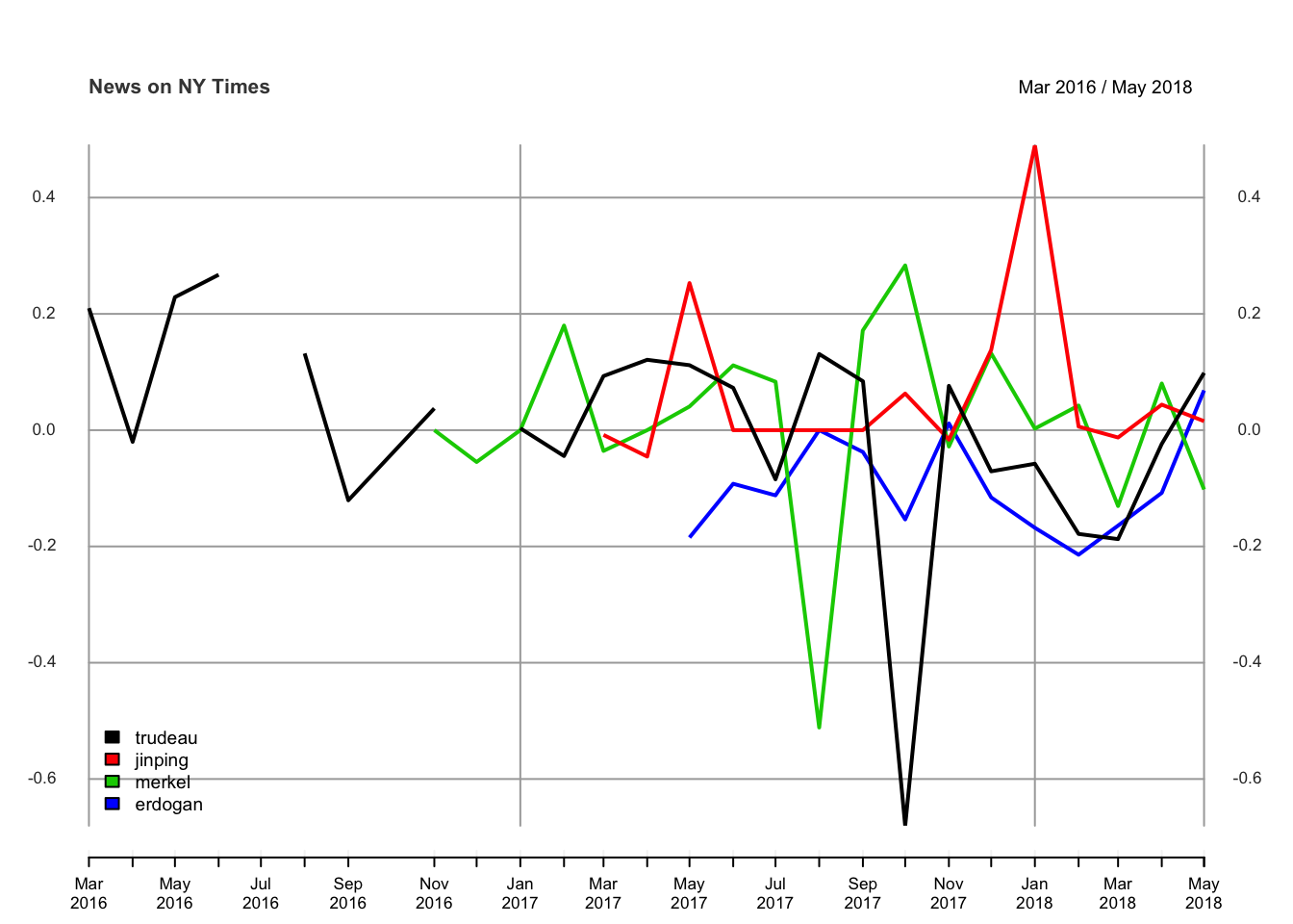
plot.xts(leaders_all, screens = factor(1, 1), auto.legend = TRUE,legend.loc = "bottomleft", main = "News on NY Times")Findings
The following plot illustrates the sentiments of the retrieved articles from the New York Times, in monthly frequency. Here, I included again the 4 leaders. Chinese leader Xi Jinping has been resulted by the highest score amongst all leaders. The correlation analysis can also be done simply. However I wanted to omit that basic stuff. It seems not a big deal. But Erdogan and Trudeau have over 50% of positive correlation. Meanwhile, Merkel and Erdogan have over 50% of negative correlation over the time between 2016 and 2018.
In order to make a dynamic plot, there are some ways provided by various packages. One of them is plotly package and you can find the plotly code below:
#devtools::install_github("ropensci/plotly")
library(plotly)

leaders_all_df <- round(as.data.frame(leaders_all),2)

leaders_all_df$date <- as.Date(as.yearmon(rownames(leaders_all_df), format = "%b %Y"))

p <- plot_ly()
for(i in 1:length(leaders_)){
  p <- add_trace(p, x = leaders_all_df$date, y = leaders_all_df[,i], mode = "lines",
                 line = list(color = rainbow(ncol(leaders_all_df)-1)[i]),
                 name = strsplit(leaders_[i], "\\W+")[[1]][length(strsplit(leaders_[i], "\\W+")[[1]])],
                 text = strsplit(leaders_[i], "\\W+")[[1]][length(strsplit(leaders_[i], "\\W+")[[1]])],
                 connectgaps = T,
                 showlegend = TRUE)
}


p <- p %>% layout(xaxis = list(title = ''),
             yaxis = list(title = 'Score'),
             legend = list(orientation = 'h'))

p
The dynamic results are below. You may use the buttons, which are provided by plotly, to modify your dynamic graph.
Reminder for the legend: One-click omits the variable, double-click keeps only the clicked variable
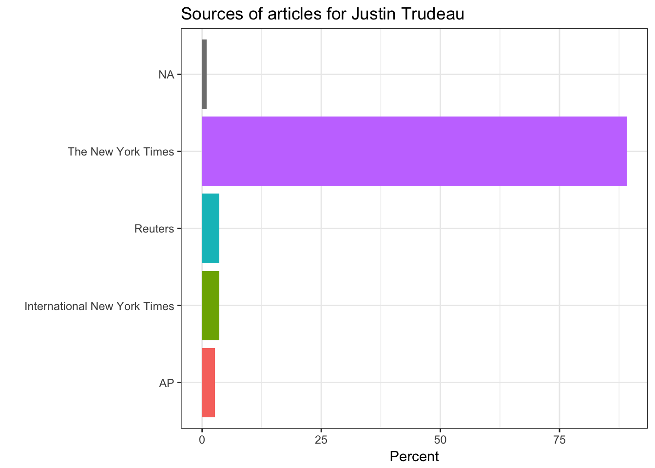
Features of Articles
In this part of the post, the features of the articles are illustrated only about Justin Trudeau. Sources of the articles, showing where the articles mostly originated from, such as the New York Times, Reuters, Associated Press, and so on. The section part illustrates which part of the New York Times does include the article. Type of material part is clear and pointing the type of the article. Lastly, the byline origin part is plotting the original author or the news agency of the news.
# Let us try only for Justin Trudeau
# For sure, you can define another word instead of a leader
# Source
require(rlang)
require(dplyr)

i <- 1
name_ <- as.character(tolower(strsplit(leaders_[i], "\\W+")[[1]][length(strsplit(leaders_[i], "\\W+")[[1]])]))

chooseOne = function(question){
  get(name_) %>%
    filter(!UQ(sym(question)) == "") %>%
    group_by_(question) %>%
    summarise(count = n()) %>%
    mutate(percent = (count / sum(count)) * 100) %>%
    arrange(desc(count))
}

the_names <- colnames(get(name_))[(c(2,3,10:12,15,19,20,25))]
news_list <- lapply(the_names, function(x) chooseOne(x))
# Source extraction
get(name_) %>%
group_by(response.docs.source) %>%
summarize(count=n()) %>%
mutate(percent = (count / sum(count))*100) %>%
ggplot() +
geom_bar(aes(y=percent, x=response.docs.source, fill=response.docs.source), stat = "identity")+
coord_flip() +
labs(x = "",y = "Percent") +
ggtitle(paste("Sources of articles for",leaders_[i])) +
theme_bw() +
theme(legend.position="none")
# Section extraction
gg_section <- get(name_) %>%
  filter(!UQ(sym('response.docs.section_name')) == "") %>%
  group_by(response.docs.section_name) %>%
  summarize(count=n()) %>%
  mutate(percent = (count / sum(count))*100) %>%
  ggplot() +
  geom_bar(aes(y=percent, x=response.docs.section_name, fill=response.docs.section_name), stat = "identity") + coord_flip() +
  labs(x = "",y = "Percent") +
  ggtitle(paste("Sections of the News for",leaders_[i])) +
  theme_bw() +
  theme(legend.position="none")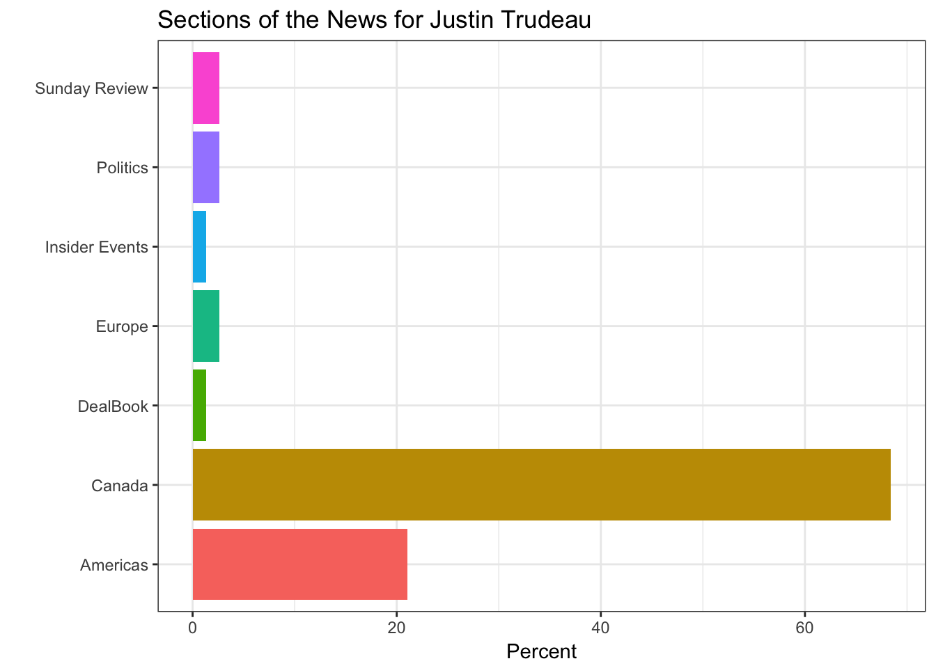
# Type of material extraction
get(name_) %>%
  group_by(response.docs.type_of_material) %>%
  summarize(count=n()) %>%
  mutate(percent = (count / sum(count))*100) %>%
  ggplot() +
  geom_bar(aes(y=percent, x=response.docs.type_of_material, fill=response.docs.type_of_material), stat = "identity") +
  coord_flip() +
  labs(x = "Type of Material",y = "Percent") +
  ggtitle(paste("Type of Material for",leaders_[i])) +
  theme_bw() +
  theme(legend.position="none")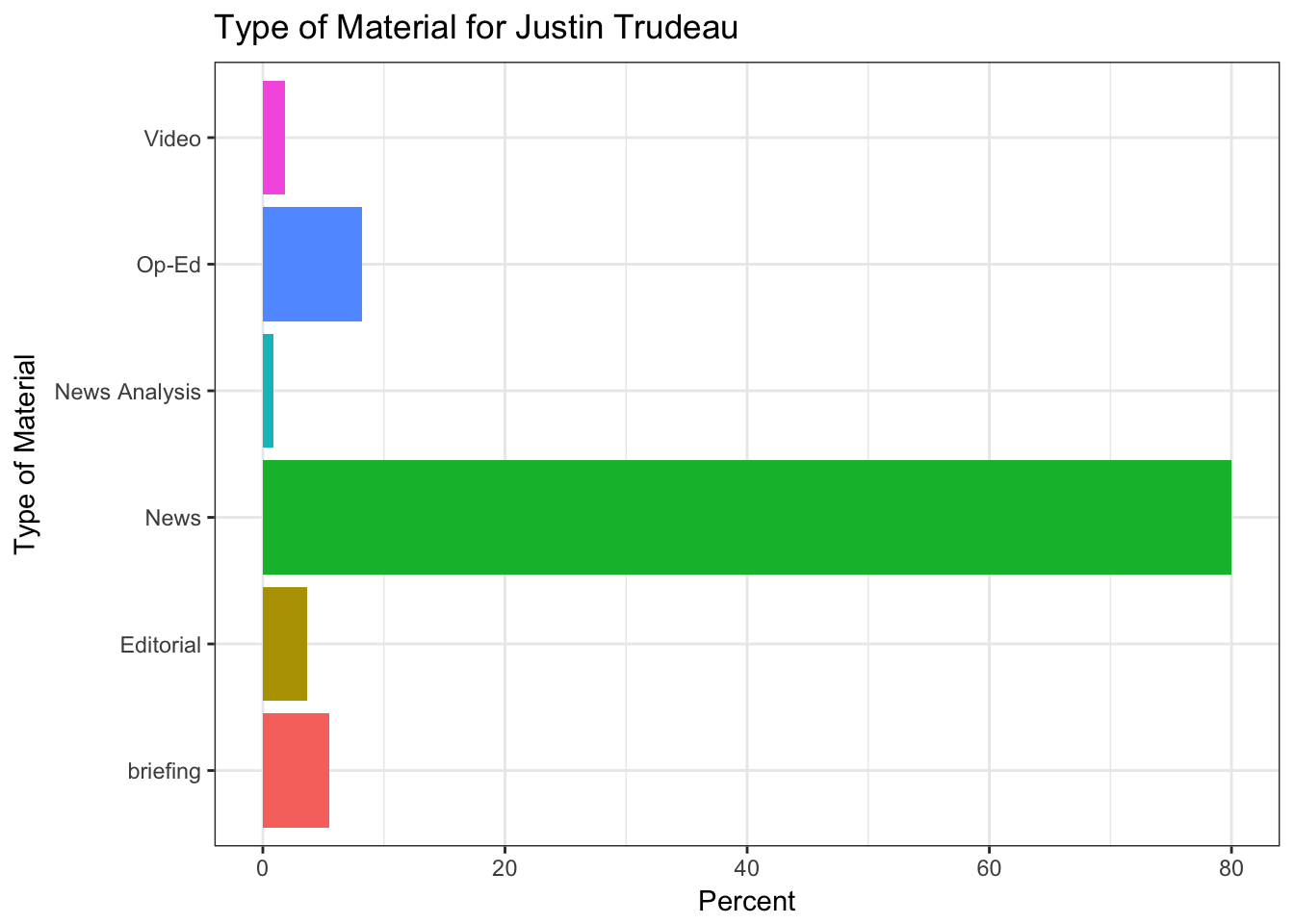
#Byline extraction
byline_ <- chooseOne('response.docs.byline.original')

head(byline_,10) %>%
  ggplot() +
  geom_bar(aes(y=percent, x=response.docs.byline.original, fill=response.docs.byline.original),
           stat = "identity") + coord_flip() +
  labs(x = "Byline",y = "Percent") +
  ggtitle(paste("Byline Origin for",leaders_[i])) +
  theme_bw() +
  theme(legend.position="none")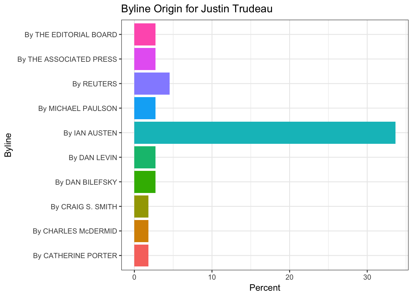
Keyword Extraction
In this part, an amazing NLP package, udpipe is going to help us. You can reach for more information about the package, you can visit the author’s website. Moreover, you can find the package in CRAN repository. We use this package here, in order to extract the most frequent nouns, to define frequently following adjective+noun structures. Then the rapid automatic keyword extraction (RAKE) feature of this package, gives more hint about the keyword extraction. Finally, I an going to show how to use a sequence of POS tags (noun phrases / verb phrases). It is a simple introduction for Part-of-Speech tagging concept.
This part of the work will be held only for the news about Chinese leader Xi Jinping. Initially, I fetch the udpipe model file from their website and I loaded the model into R.
ps: You can use this packages for many languages.
require(lattice)
require(udpipe)

# Let us try only for Xi Jinping
i <- 2
name_ <- as.character(tolower(strsplit(leaders_[i], "\\W+")[[1]][length(strsplit(leaders_[i], "\\W+")[[1]])]))

ud_model <- udpipe_download_model(language = "english") # If you download once, you would not need repeat this process again
ud_model <- udpipe_load_model("...") # Path of the downloaded file needed
x <- as.data.frame(udpipe_annotate(ud_model, x = get(name_)$response.docs.snippet))
stats <- subset(x, upos %in% "NOUN")
stats <- txt_freq(x = stats$lemma)
stats$key <- factor(stats$key, levels = rev(stats$key)) # Making a factor vector
barchart(key ~ freq, data = head(stats, 15),
col = "light green", main = paste("Most occurring nouns for", leaders_[i]), xlab = "Freq")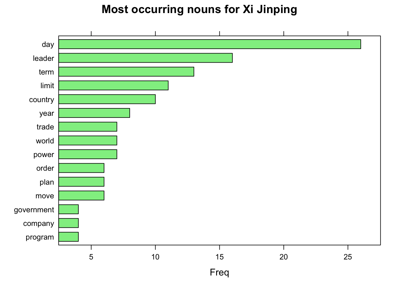
The most frequent nouns are “day”, “leader” and “term”; probably indicating the presidential due date of the China in last year. Now we can jump to word collocation section. Here I try the condition of nouns following by an adjective in the same sentence, not in the same sentence, and while the words follow one another even if we would skip 2 words in between. These examples can also be found in the package author’s website.
# Collocation example
stats <- keywords_collocation(x = x,
                              term = "token", group = c("doc_id", "paragraph_id", "sentence_id"),
                              ngram_max = 4)
## How frequent do words occur in the same sentence, in this case only nouns or adjectives
stats <- cooccurrence(x = subset(x, upos %in% c("NOUN", "ADJ")),
                      term = "lemma", group = c("doc_id", "paragraph_id", "sentence_id"))
## How frequent do words follow one another
stats <- cooccurrence(x = x$lemma,
                      relevant = x$upos %in% c("NOUN", "ADJ"))
## How frequent do words follow one another even if we would skip 2 words in between
stats <- cooccurrence(x = x$lemma,
                      relevant = x$upos %in% c("NOUN", "ADJ"), skipgram = 2)
head(stats)

library(textrank)
library(igraph)
library(ggraph)
library(ggplot2)

ggraph(graph_from_data_frame(head(stats, 20)), layout = "fr") +
  geom_edge_link(aes(width = cooc, edge_alpha = cooc), edge_colour = "pink") +
  geom_node_text(aes(label = name), col = "darkgreen", size = 4) +
  theme_graph(base_family = "Arial Narrow") +
  theme(legend.position = "none") +
  labs(title = "Cooccurrences within 3 words distance", subtitle = paste0(leaders_[i],", Nouns & Adjective"))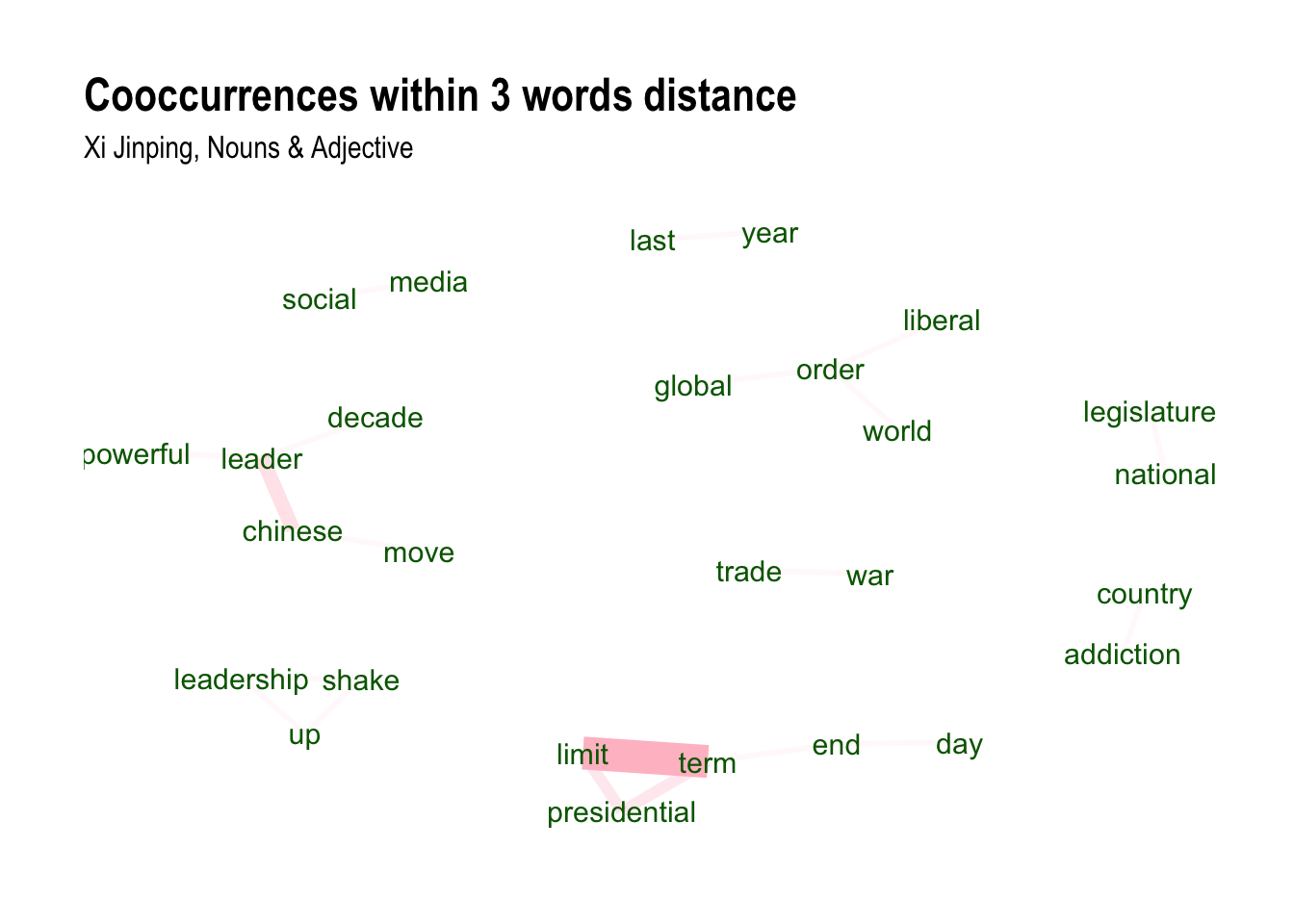
#Rapid Automatic Keyword Extraction
stats <- keywords_rake(x = x,
                       term = "token", group = c("doc_id", "paragraph_id", "sentence_id"),
                       relevant = x$upos %in% c("NOUN", "ADJ"),
                       ngram_max = 4)

head(subset(stats, freq > 3))

stats$key <- factor(stats$keyword, levels = rev(stats$keyword))

barchart(key ~ rake, data = head(subset(stats, freq > 3), 20), col = "red",
                     main = paste("Keywords identified by RAKE for", leaders_[i]),
                     xlab = "Rake")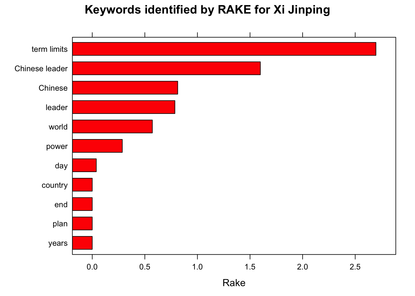
# Simple noun phrases (a adjective+noun, pre/postposition, optional determiner and another adjective+noun)
# Using a sequence of POS tags (noun phrases / verb phrases)
x$phrase_tag <- as_phrasemachine(x$upos, type = "upos")
stats <- keywords_phrases(x = x$phrase_tag, term = tolower(x$token),
                          pattern = "(A|N)*N(P+D*(A|N)*N)*",
                          is_regex = TRUE, detailed = FALSE)
stats <- subset(stats, ngram > 1 & freq > 3)
stats$key <- factor(stats$keyword, levels = rev(stats$keyword))


stats <- stats[order(stats$freq,decreasing = T),]
stats$key <- factor(stats$key, levels = rev(stats$key))

barchart(key ~ freq, data = head(stats, 20), col = "cyan",
                    main = paste0("Keywords - simple noun phrases for ",leaders_[i]), xlab = "Frequency")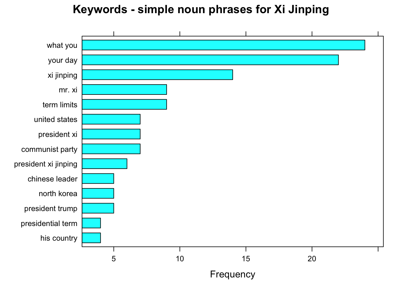
Cultural Difference and LASSO
Ege Or & Sun Huilin, 22 July 2018
Psychological research about cross-cultural differences and their statistical proof by LASSO regression.